[
Simulated Annealing Using FastAI Libraries
In this blog post, we’ll explore how to use simulated annealing to optimize the learning rate schedule for deep neural network training using FastAI libraries. We’ll extend the LRFinder class to include cosine annealing and use the Metric class to calculate accuracy during training.
What is Simulated Annealing?
Simulated annealing is a global optimization technique that uses a probabilistic approach to find the optimal solution for a given problem. It’s inspired by the annealing process in metallurgy, where a material is heated and then cooled slowly to remove defects and achieve a more stable state.
In the context of deep learning, simulated annealing can be used to optimize the learning rate schedule for a model. The idea is to start with an initial learning rate, gradually decrease it over time, and occasionally pause or “anneal” the learning process to allow the model to converge better.
Cosine Annealing
One popular variant of simulated annealing is cosine annealing. Instead of decreasing the learning rate linearly over time, cosine annealing uses a cosine function to gradually reduce the learning rate. This allows the model to slow down its descent into the optimum and helps prevent getting stuck in local minima.
Here’s the formula for cosine annealing:
\[ CurrentLF = StartingRate * (Maxixum(cos(pi * (1 - CurrentSteps/TotalSteps))) \]
where StartingRate is the initial learning rate, CurrentLF is the learning rate calcuated at the CurrentSteps, and TotalSteps is the total number of steps.
Implementing Cosine Annealing in FastAI
To incorporate cosine annealing into our FastAI workflow, we’ll extend the LRFinder class and add a new method called cosine_annealing. Here’s the updated code:
class LRFinderCB(Callback):
def __init__(self, lr_mult=1.3):
fc.store_attr()
def before_fit(self, learn):
self.epochs, self.lrs,self.losses = [],[], []
self.min = math.inf
self.t_iter = len(learn.dls.train) * learn.n_epochs


def after_batch(self, learn):
if not learn.training: raise CancelEpochException()
self.lrs.append(learn.opt.param_groups[0]['lr'])
loss = to_cpu(learn.loss)
c_iter = learn.iter
self.losses.append(loss)
self.epochs.append(c_iter)
if loss < self.min: self.min = loss
if loss > self.min*2: raise CancelFitException()
for g in learn.opt.param_groups: g['lr'] *= self.lr_mult
g['lr'] = g['lr']*max(np.cos((1-4.0*np.pi*(c_iter / self.t_iter))),1.0)
The Metric class is used to calculate how far our predictions will be from the targets.
class Metric:
def __init__(self):
self.reset()


def reset(self):
self.vals, self.ns = [], []


def add(self, inp, targ=None, n=1):
self.last = self.calc(inp, targ)
self.vals.append(self.last)
self.ns.append(n)


@property
def value(self):
ns = tensor(self.ns)
return (tensor(self.vals) * ns).sum() / ns.sum()


def calc(self, inps, targs):
return (inps == targs).float().mean()


class Accuracy(Metric):
def calc(self, inps, targs):
return (inps == targs).float().mean()
Since the LRFinder object has the cosine annealer integrated. All we did was add the cosine function as a factor so that the learning rate is adjusted after every batch.
Using the Metric Class to Calculate Accuracy
To calculate accuracy during training, we can use the Metric class provided by FastAI. This class allows us to compute a metric over a dataset and print it out at each epoch.
We’ll create a custom accuracy Metric class that calculates the accuracy of our model on the validation set by comparing how far apart our predictions are from the validation values. Here’s how to do it:
class Metric:
def __init__(self): self.reset()
def reset(self): self.vals,self.ns = [],[]
def add(self, inp, targ=None, n=1):
self.last = self.calc(inp, targ)
self.vals.append(self.last)
self.ns.append(n)
@property
def value(self):
ns = tensor(self.ns)
return (tensor(self.vals)*ns).sum()/ns.sum()
def calc(self, inps, targs): return inps
We make the class callable by creating a function called Accuracy(Metric) Accuracy takes in two tensors, pred and validate, which represent the predicted outputs and the true labels, respectively. It then computes the accuracy by counting the number of correctly predicted samples and dividing it by the total number of samples.
class Accuracy(Metric):
def calc(self, inps, targs): return (inps==targs).float().mean()
We can now register this metric with FastAI’s CallbackList to get the accuracy and loss of each epoch:
from fastai.callbacks import CallbackList


cb_list = CallbackList()
cb_list.insert(Accuracy())
With this callback list, FastAI will call the Accuracy metric at each epoch and print out the accuracy.
The Training Model
Let’s take an inside peak what our single-layer model is doing. By looking at the training call back we can see the architecture of our model.
class TrainCB(Callback):
def __init__(self, n_inp=1): self.n_inp = n_inp
def predict(self, learn): learn.preds = learn.model(*learn.batch[:self.n_inp])
def get_loss(self, learn): learn.loss = learn.loss_func(learn.preds, *learn.batch[self.n_inp:])
def backward(self, learn): learn.loss.backward()
def step(self, learn): learn.opt.step()
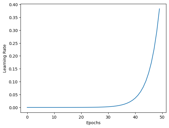
def zero_grad(self, learn): learn.opt.zero_grad()This training loop will train the model for 50 epochs, computing the accuracy at each batch pass using the Accuracy metric and updating the learning rate. Let’s start by looking at our loss and learning rates with the momentum learner on its own without cosine annealing. In figure 1 we can see that the learning rate starts to take off after 25 epochs.
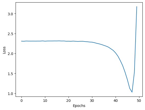
posts/2023-08-28- FastAI Cosine Annealer/assets In Figure 2 we see that the loss is minimized at approximately the 47th epoch.
Let’s add a cosine factor:
max(np.cos((1-4.0*np.pi*(c_iter / self.t_iter))),1.0)
so that the learning rate is forced over a smooth 1 to 0 set of factors.
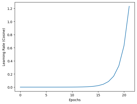
Figure 3 demonstrates how the learning rate is smoothly ramped up from zero after the 13th epoch which is an improvement over the 25 we achieve without annealing.
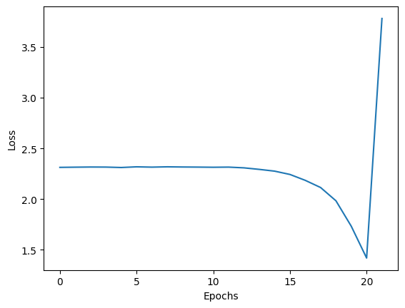
Looking at Figure 4 we can see a further improvement in finding the minimum loss at the 20th epoch which is less than half as many passes as needed without it.
And that’s it! With these few lines of code, you’ve implemented a powerful annealing function and integrated it into the FastAI learner.
Conclusion
In this tutorial, we learned how to implement cosine annealing and accuracy calculation in a FastAI training loop. By extending the LRFinder class and creating a custom Accuracy metric, we were able to create a complete training loop that adapts the learning rate during training and prints out the accuracy at each epoch.
With this knowledge, you can now apply these techniques to your own deep-learning projects and improve the performance of your models.